42 excel pie chart add labels
› pie-chart-examplesPie Chart Examples | Types of Pie Charts in Excel with Examples It is similar to Pie of the pie chart, but the only difference is that instead of a sub pie chart, a sub bar chart will be created. With this, we have completed all the 2D charts, and now we will create a 3D Pie chart. 4. 3D PIE Chart. A 3D pie chart is similar to PIE, but it has depth in addition to length and breadth. Data Labels in Excel Pivot Chart (Detailed Analysis) Add a Pivot Chart from the PivotTable Analyze tab. Then press on the Plus right next to the Chart. Next open Format Data Labels by pressing the More options in the Data Labels. Then on the side panel, click on the Value From Cells. Next, in the dialog box, Select D5:D11, and click OK.
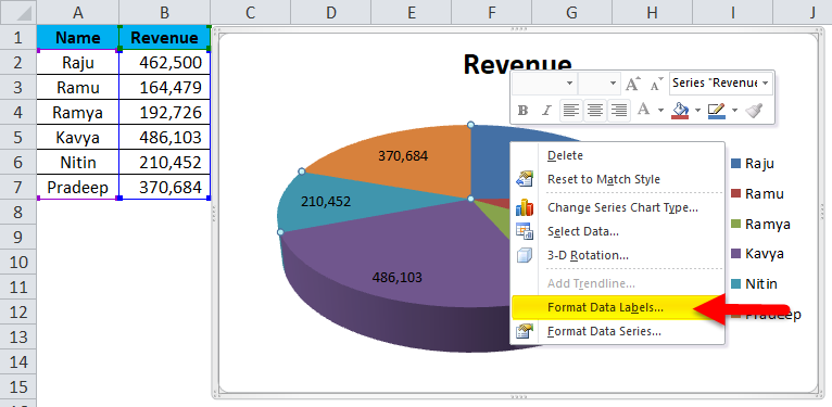
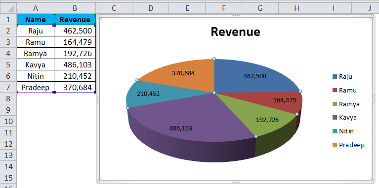
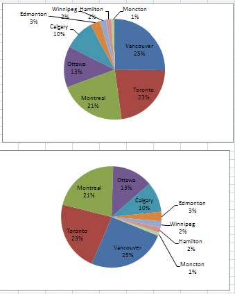
Excel Pie Chart - How to Create & Customize? (Top 5 Types) We will customize the Pie Chart in Excel by Adding Data Labels. Scenario 1: The procedure to add data labels are as follows: Click on the Pie Chart > click the ' + ' icon > check/tick the " Data Labels " checkbox in the " Chart Element " box > select the " Data Labels " right arrow > select the " Outside End " option. We get the following output.
Excel pie chart add labels
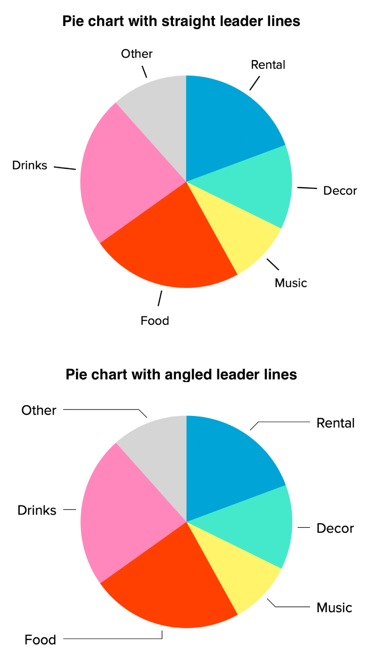
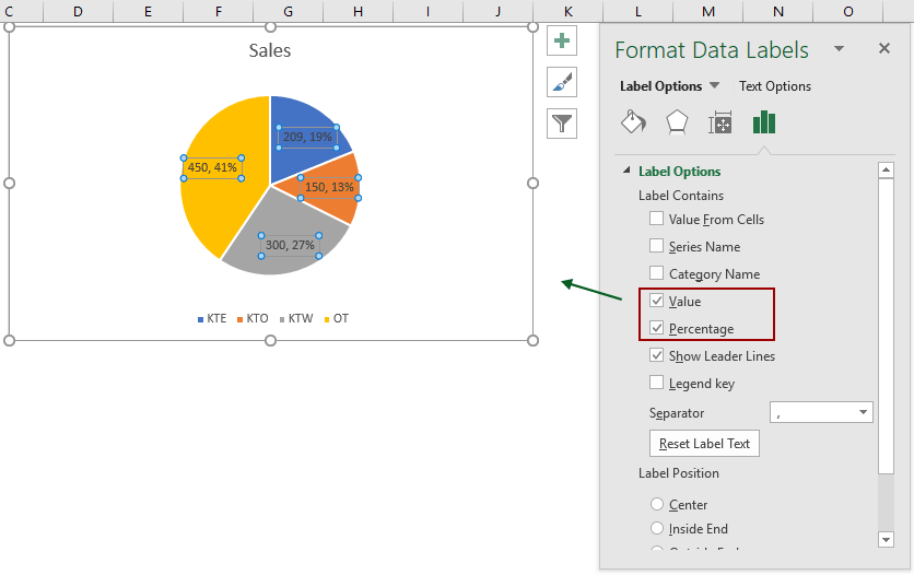
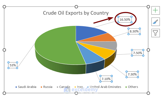
How to Show Percentage and Value in Excel Pie Chart - ExcelDemy Download Practice Workbook. Step by Step Procedures to Show Percentage and Value in Excel Pie Chart. Step 1: Selecting Data Set. Step 2: Using Charts Group. Step 3: Creating Pie Chart. Step 4: Applying Format Data Labels. Conclusion. Related Articles. How to display leader lines in pie chart in Excel? - ExtendOffice To display leader lines in pie chart, you just need to check an option then drag the labels out. 1. Click at the chart, and right click to select Format Data Labels from context menu. 2. In the popping Format Data Labels dialog/pane, check Show Leader Lines in the Label Options section. See screenshot: 3. › charts › gauge-templateExcel Gauge Chart Template - Free Download - How to Create Step #7: Add the pointer data into the equation by creating the pie chart. Step #8: Realign the two charts. Step #9: Align the pie chart with the doughnut chart. Step #10: Hide all the slices of the pie chart except the pointer and remove the chart border. Step #11: Add the chart title and labels.
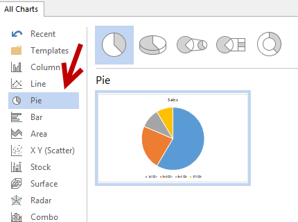
Excel pie chart add labels. › pie-chart-excelHow to Create a Pie Chart in Excel | Smartsheet Aug 27, 2018 · To create a pie chart in Excel 2016, add your data set to a worksheet and highlight it. Then click the Insert tab, and click the dropdown menu next to the image of a pie chart. Select the chart type you want to use and the chosen chart will appear on the worksheet with the data you selected. Pie Chart in Excel - Inserting, Formatting, Filters, Data Labels The total of percentages of the data point in the pie chart would be 100% in all cases. Consequently, we can add Data Labels on the pie chart to show the numerical values of the data points. We can use Pie Charts to represent: ratio of population of male and female of a country. proportion of online/offline payment modes of a local car rental ... How to Make a Pie Chart in Excel & Add Rich Data Labels to The Chart! Creating and formatting the Pie Chart 1) Select the data. 2) Go to Insert> Charts> click on the drop-down arrow next to Pie Chart and under 2-D Pie, select the Pie Chart, shown below. 3) Chang the chart title to Breakdown of Errors Made During the Match, by clicking on it and typing the new title. › make-pie-chart-in-excelPie Charts in Excel - How to Make with Step by Step Examples These percentages will appear as data labels on the pie chart. For adding such data labels, right-click the pie chart and choose “add data labels” from the context menu. • Method 2–Enter numbers as is in the series and let Excel convert them to percentages. Once converted, the numbers and percentages will appear as data labels on the ...
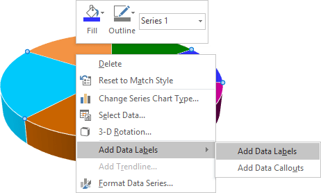
› documents › excelHow to create a pie chart for YES/NO answers in Excel? 4. Now the pivot chart is created. Right click the series in the pivot chart, and select Change Series Chart Type from the context menu. See screenshot: 5. In the Change Chart Type dialog, please click Pie in the left bar, click to highlight the Pie chart in the right section, and click the OK button. See screenshot: Excel custom pie chart labels - Microsoft Community Answer HansV MVP MVP Replied on July 8, 2019 Report abuse Specify (space) as Separator in the Data Labels. Set the Number format of the data labels to Custom, and specify (0%) as Type. --- Kind regards, HansV 6 people found this reply helpful · Was this reply helpful? Yes No Replies (1) Change the format of data labels in a chart To get there, after adding your data labels, select the data label to format, and then click Chart Elements > Data Labels > More Options. To go to the appropriate area, click one of the four icons ( Fill & Line, Effects, Size & Properties ( Layout & Properties in Outlook or Word), or Label Options) shown here. Add or remove data labels in a chart - support.microsoft.com In the upper right corner, next to the chart, click Add Chart Element > Data Labels. To change the location, click the arrow, and choose an option. If you want to show your data label inside a text bubble shape, click Data Callout. To make data labels easier to read, you can move them inside the data points or even outside of the chart.
How to add data labels in excel to graph or chart (Step-by-Step) Add data labels to a chart. 1. Select a data series or a graph. After picking the series, click the data point you want to label. 2. Click Add Chart Element Chart Elements button > Data Labels in the upper right corner, close to the chart. 3. Click the arrow and select an option to modify the location. 4. Edit titles or data labels in a chart - support.microsoft.com On a chart, click the label that you want to link to a corresponding worksheet cell. On the worksheet, click in the formula bar, and then type an equal sign (=). Select the worksheet cell that contains the data or text that you want to display in your chart. You can also type the reference to the worksheet cell in the formula bar. Creating Pie Chart and Adding/Formatting Data Labels (Excel) Creating Pie Chart and Adding/Formatting Data Labels (Excel) › documents › excelHow to create pie of pie or bar of pie chart in Excel? And you will get the following chart: 4. Then you can add the data labels for the data points of the chart, please select the pie chart and right click, then choose Add Data Labels from the context menu and the data labels are appeared in the chart. See screenshots: And now the labels are added for each data point. See screenshot: 5.
Change the look of chart text and labels in Numbers on Mac ...
How to Create and Format a Pie Chart in Excel - Lifewire Select the plot area of the pie chart. Right-click the chart. Select Add Data Labels . Select Add Data Labels. In this example, the sales for each cookie is added to the slices of the pie chart. Change Colors When a chart is created in Excel, or whenever an existing chart is selected, two additional tabs are added to the ribbon.
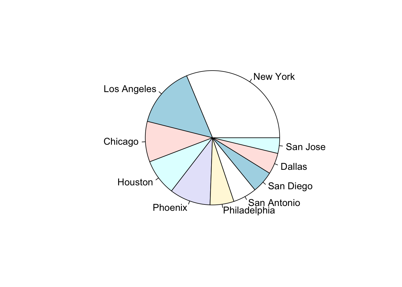
Chapter 9 Pie Chart | Basic R Guide for NSC Statistics
How to insert data labels to a Pie chart in Excel 2013 - YouTube This video will show you the simple steps to insert Data Labels in a pie chart in Microsoft® Excel 2013. Content in this video is provided on an "as is" basis with no express or implied...

How to create pie of pie or bar of pie chart in Excel?
Add or remove data labels in a chart - support.microsoft.com Click the data series or chart. To label one data point, after clicking the series, click that data point. In the upper right corner, next to the chart, click Add Chart Element > Data Labels. To change the location, click the arrow, and choose an option. If you want to show your data label inside a text bubble shape, click Data Callout.
Pie Chart in Excel | How to Create Pie Chart | Step-by-Step ...
How to show percentage in pie chart in Excel? - ExtendOffice Please do as follows to create a pie chart and show percentage in the pie slices. 1. Select the data you will create a pie chart based on, click Insert > I nsert Pie or Doughnut Chart > Pie. See screenshot: 2. Then a pie chart is created. Right click the pie chart and select Add Data Labels from the context menu. 3.

Change the format of data labels in a chart
excel - Pie Chart VBA DataLabel Formatting - Stack Overflow sub updatechartformat () with activesheet.chartobjects ("chart 4") .activate with .chart.seriescollection (1).datalabels .showpercentage = true .separator = "" & chr (10) & "" end with end with with activesheet.chartobjects ("chart 1") .activate with .chart.seriescollection (1).datalabels .showpercentage = true .showvalue = false …
Pie Chart in Excel | How to Create Pie Chart | Step-by-Step ...
Pie Charts in Excel - How to Make with Step by Step Examples Let us create each Excel pie chart one by one with the help of examples. 2-D Pie Chart. A 2-D (two-dimensional) pie chart is frequently used in Excel. It is a standard pie chart that displays one slice for each data point. The bigger the number (or data point) represented by the slice, the larger the area under it. ... Add data labels and data ...
EXCEL Charts: Column, Bar, Pie and Line
Pie Chart in Excel | How to Create Pie Chart - EDUCBA Step 1: Select the data to go to Insert, click on PIE, and select 3-D pie chart. Step 2: Now, it instantly creates the 3-D pie chart for you. Step 3: Right-click on the pie and select Add Data Labels. This will add all the values we are showing on the slices of the pie.

Change the format of data labels in a chart
How to Show Percentage in Excel Pie Chart (3 Ways) Read More: Add Labels with Lines in an Excel Pie Chart (with Easy Steps) 2.2 Using Context Menu. We can also use the context menu to display percentages in a pie chart. Let's follow the steps below. Steps: Right-click on the pie chart to open the context menu. Choose the Add Data Labels ;
Excel 3-D Pie charts - Microsoft Excel 365
support.microsoft.com › en-us › officeAdd a pie chart - support.microsoft.com Click Insert > Insert Pie or Doughnut Chart, and then pick the chart you want. Click the chart and then click the icons next to the chart to add finishing touches: To show, hide, or format things like axis titles or data labels, click Chart Elements . To quickly change the color or style of the chart, use the Chart Styles .

How to Make Pie Chart with Labels both Inside and Outside ...
› charts › gauge-templateExcel Gauge Chart Template - Free Download - How to Create Step #7: Add the pointer data into the equation by creating the pie chart. Step #8: Realign the two charts. Step #9: Align the pie chart with the doughnut chart. Step #10: Hide all the slices of the pie chart except the pointer and remove the chart border. Step #11: Add the chart title and labels.

How to Make Pie Chart with Labels both Inside and Outside ...
How to display leader lines in pie chart in Excel? - ExtendOffice To display leader lines in pie chart, you just need to check an option then drag the labels out. 1. Click at the chart, and right click to select Format Data Labels from context menu. 2. In the popping Format Data Labels dialog/pane, check Show Leader Lines in the Label Options section. See screenshot: 3.
How to Make a Pie Chart in Google Sheets - How To NOW
How to Show Percentage and Value in Excel Pie Chart - ExcelDemy Download Practice Workbook. Step by Step Procedures to Show Percentage and Value in Excel Pie Chart. Step 1: Selecting Data Set. Step 2: Using Charts Group. Step 3: Creating Pie Chart. Step 4: Applying Format Data Labels. Conclusion. Related Articles.
How to ☝️Make a Pie Chart in Excel (Free Template ...
Help Online - Quick Help - FAQ-1017 How to recover the ...

How to Create a Pie Chart in Excel | Smartsheet

Vizible Difference: Labeling Inside Pie Chart
Pie Chart Rounding in Excel - Peltier Tech

Office: Display Data Labels in a Pie Chart

Interactive R pie chart labels. Statistics for Ecologists ...

Add or remove data labels in a chart
information graphics - How to display data labels in ...

How to Show Percentage in Pie Chart in Excel? - GeeksforGeeks

EXCEL Charts: Column, Bar, Pie and Line

How-to Make a WSJ Excel Pie Chart with Labels Both Inside and ...
How to make a pie chart in Excel
Excel Pie Chart Secrets - TechTV Articles - MrExcel Publishing
How to show percentage in pie chart in Excel?
Excel 3-D Pie charts - Microsoft Excel 2016

How to Make a Pie Chart in Excel - All Things How

How to Create a 3D Pie Chart in Excel (with Easy Steps)

How to fix wrapped data labels in a pie chart | Sage Intelligence
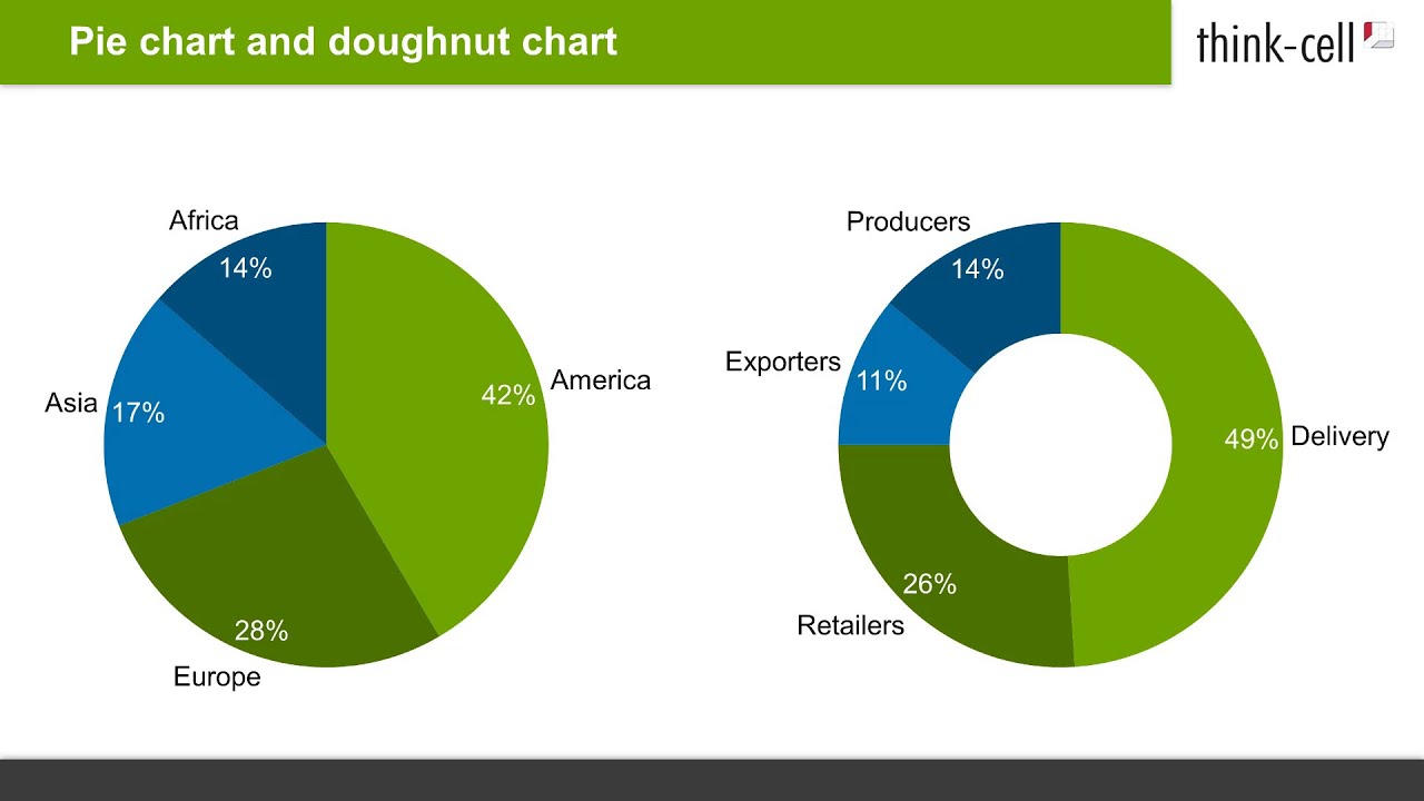
How to create pie charts and doughnut charts in PowerPoint ...
Create a Pie Chart in Excel (Easy Tutorial)

how to see more than 5 labels in pie chart in tableau - Stack ...
Office: Display Data Labels in a Pie Chart
Appian Community

Custom data labels in a chart

How to Create a Pie Chart in Excel - Displayr

Change the format of data labels in a chart

How to Make Excel Pie Chart Examples Videos ◔

Pie Charts in Excel - How to Make with Step by Step Examples
Add Labels with Lines in an Excel Pie Chart (with Easy Steps)
Post a Comment for "42 excel pie chart add labels"