44 excel chart multiple data labels

Macro to extract data from a chart in Excel - Office | Microsoft Docs In Excel 2007, click the Data tab, click Edit Links in the Connenctions group, and then click Change Source. In the Source File box, select the link to change, and then click Change Source. In the Change Links dialog box, select the new file with the recovered data and chart, and then click OK. If you receive the following error message Format Data labels to get integers. - Microsoft Community You have to specify the series number and the data label sequence number. This code worked to revalue the second data label on series 1 in a sample chart I opened. '--- Sub test () ActiveSheet.ChartObjects (1).Chart.SeriesCollection (1).DataLabels (2).Formula = (Range ("A15").Value * 10) End Sub '--- Nothing Left to Lose

Excel Pivot Table tutorial - Ablebits To do this, in Excel 2013 and higher, go to the Insert tab > Charts group, click the arrow below the PivotChart button, and then click PivotChart & PivotTable. In Excel 2010 and 2007, click the arrow below PivotTable, and then click PivotChart. 3. Arranging the layout of your pivot table report

Excel chart multiple data labels

Excel: Compare two columns for matches and differences - Ablebits Example 1. Compare two columns for matches or differences in the same row. To compare two columns in Excel row-by-row, write a usual IF formula that compares the first two cells. Enter the formula in some other column in the same row, and then copy it down to other cells by dragging the fill handle (a small square in the bottom-right corner of ... Excel Formula Symbols Cheat Sheet (13 Cool Tips) - ExcelDemy The formula for calculating the Area is, =A2*B2. Now place this formula in cell C2 and press enter. If you select this cell C2 again you will see a green-colored box surrounds it, this box is known as the fill handle. Now drag this fill handle box downwards to paste the formula for the entire column. How to Repeat Formula Pattern in Excel (Easiest 8 ways) Method-5: Using Power Query to Repeat Pattern. Step-01: Here, I want to complete the Total Income column by typing the formula only once. To do this you have to select as following Data Tab >> From Table/Range. Step-02: Then Create Table Dialog Box will appear. Then you have to select the whole range and click on the My table has headers option ...

Excel chart multiple data labels. One Weird Trick for Smarter Map Labels in Tableau - InterWorks Simply add a second Latitude dimension onto the rows shelf, right-click and select "dual axis." This allows you to set the mark type individually for each layer of the map. Select "Latitude (2)" and change the mark type to "Circle" as shown below. Final Tweaks The above steps will do some things to your map that aren't desirable. 12 Best Line Graph Maker Tools For Creating Stunning Line Graphs [2022 ... A line graph is a graphical representation of data to display the value of something over time. It contains X-axis and Y-axis, where both the X and Y axis are labeled according to the data types which they are representing. A line graph is created by connecting the plotted data points with a line. It is also known as a line chart. Excel - Quantitative Analysis Guide - Research Guides at New York ... Learn to create different kinds of Excel charts, from column, bar, line and pie to more recently introduced types like Treemap, Funnel, and Pareto. Plus, learn how to fine-tune your chart's color and style; add titles, labels, and legends; insert shapes, pictures, and text boxes; and pull data from multiple sources. Network Diagram Template | [Free] Network Topology Creator in Excel! This Excel template allows you to create a Network Diagram in two ways: Input all your data into the table and then create a network diagram based on the data input. Visually create a network diagram using the interactive buttons and shapes without filling the data table. Both of those methods are connected, so if you make changes in the table ...

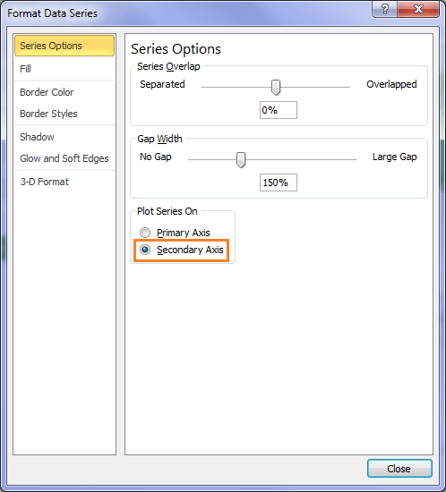
Bar Chart Series Issues - Microsoft Tech Community Bar Chart Series Issues. I have a bar chart with three series plotted against dates. The horizontal (date) axis is dynamic and so are the series, all of which use named ranges. The named ranges are working just fine, but there's a quirk about my chart that I can't figure out. With filter showing all three series together, the first one, Westpac ... Make Excel charts primary and secondary axis the same scale In the first cell create a MIN function that looks at ALL the original data points and finds the smallest number. In the last cell do the same but this time a MAX to find the biggest number out of all the data points. In E8 and E34 just equals to the adjacent cells. You now know what the scale needs to be. Insert the new series into the chart How to: Create and Modify a Chart | WinForms Controls - DevExpress You can also place a chart on a separate worksheet by creating a chart sheet (see How to: Create a Chart Sheet for details).. Add or Remove Data Series. If you did not specify the range containing chart data in the ChartCollection.Add method, you can define it later by using one of the following approaches.. Pass the required data range to the ChartObject.SelectData method. Use defined names to automatically update a chart range - Office Select cells A1:B4. On the Insert tab, click a chart, and then click a chart type. Click the Design tab, click the Select Data in the Data group. Under Legend Entries (Series), click Edit. In the Series values box, type =Sheet1!Sales, and then click OK. Under Horizontal (Category) Axis Labels, click Edit.

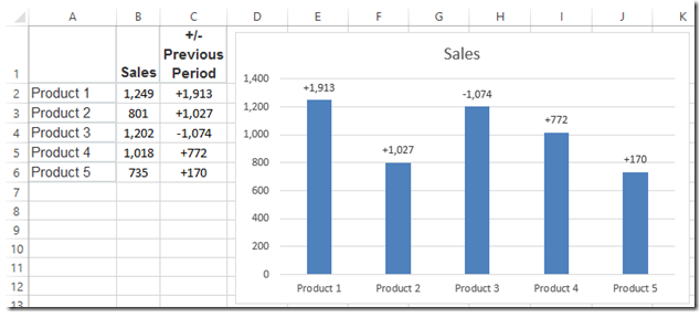
What would be a situation in which you could use an Excel chart to ... Weegy: What percentage of customer 101 buys product A, [ and what percentage of the same customer buys product B? -is a situation where you could use an Excel chart to present your data. ] Score .9771 User: What is entered into a cell that is typically numeric and can be used for calculations A. Value B. Tab C. Label D. Function Excel filtering pivot table filter/slicer across column label Excel filtering pivot table filter/slicer across column label. Hello. I have a table with the year as the column headings/labels (2009-2021) and a couple other columns with additional information that aren't a year. The rows represent the specific data for each year. I have made a pivot table and slicers for the columns with the other date but ... How to Add Axis Label to Chart in Excel - Sheetaki Method 1: By Using the Chart Toolbar Select the chart that you want to add an axis label. Next, head over to the Chart tab. Click on the Axis Titles. Navigate through Primary Horizontal Axis Title > Title Below Axis. An Edit Title dialog box will appear. In this case, we will input "Month" as the horizontal axis label. Next, click OK. What type of chart to use to compare data in Excel To do that, follow the steps below: Step-1: Right-click on the column chart whose row and column you want to change. Step-2: Click on 'Select Data' from the drop-down menu: Step-3: Click on the 'Switch/Row Column' button: Step-4: Click on the 'OK' button. The column chart will now look like the one below:

Excel Course: Inserting Graphs

How to create and use two-input data tables in Excel - Office Right-click cell B14, and then click Format Cells. Click the Number tab. In the Category list, click Custom. In the Type box, type "" (two quotation marks). Click OK. References For more information about how to use data tables, view the following articles: Calculate multiple results by using a data table

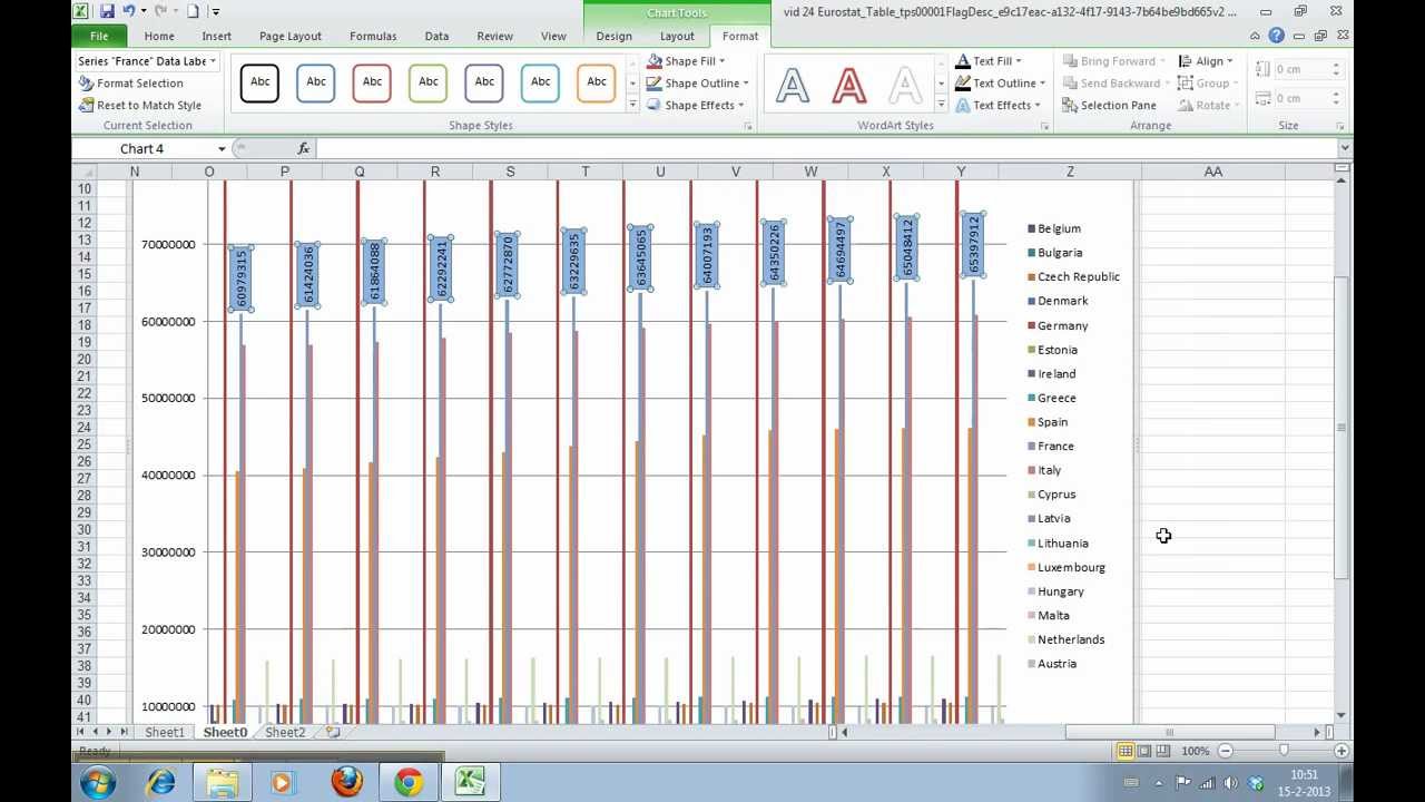
Multiple Series in One Excel Chart - Peltier Tech Blog

Display more digits in trendline equation coefficients - Office Method 1: Microsoft Office Excel 2007 Open the worksheet that contains the chart. Right-click the trendline equation or the R-squared text, and then click Format Trendline Label. Click Number. In the Categorylist, click Number, and then change the Decimal placessetting to 30 or less. Click Close.

32 What Is A Data Label In Excel - Labels Design Ideas 2020

50 Excel Shortcuts That You Should Know in 2022 - Simplilearn First, let's create a pivot table using a sales dataset. In the image below you can see that we have a pivot table to summarize the total sales for each subcategory of the product under each category. Fig: Pivot table using sales data 46. To group pivot table items Alt + Shift + Right arrow

Advanced Graphs Using Excel : Strip plot / Strip Chart in Excel using RExcel

Date Axis in Excel Chart is wrong • AuditExcel.co.za In order to do this you just need to force the horizontal axis to treat the values as text by right clicking on the horizontal axis, choose Format Axis Change Axis Type to be Text Note that you immediately lose the scaling options and the date scale puts in exactly what is in the data, onto the horizontal axis.

Treemap Excel Charts: The Perfect Tool for Displaying Hierarchical Data

How to: Display and Format Data Labels - DevExpress To display value labels, set the DataLabelBase.ShowValue property of the DataLabelOptions object to true. Series name. Series labels identify data series to which the data points in the chart belong. Most series include multiple data points, so the same name will be repeated for all data points in the series, which is probably overkill.

Excel Custom Chart Labels • My Online Training Hub

Excel table styles and formatting: how to apply, change and remove On the Design tab, in the Table Styles group, click the More button. Underneath the table style templates, click Clear. Tip. To remove a table but keep data and formatting, go to the Design tab Tools group, and click Convert to Range. Or, right-click anywhere within the table, and select Table > Convert to Range.

Can highcharts generate a 3d column chart like this? - Highcharts official support forum

Excel Pivot Table DrillDown Show Details Right-click the pivot table's worksheet tab, and then click View Code. That opens the Visual Basic Explorer (VBE). Paste the copied code onto the worksheet module, below the Option Explicit line (if there is one), at the top of the code module (optional) Paste the copied code onto the worksheet module for any other pivot tables in your workbook

How to Make Excel Charts More Intuitive by Adding Data Labels and Tables - Data Recovery Blog

How to Format Number to Millions in Excel (6 Ways) Let's take a look at the steps below. STEPS: To begin with, select the cell where we want to change the format. So, we select cell E5. Now, we write the formula below. =TEXT (D5,"#,##0,,")&"M" As we take the value from D5, we write D5 in the formula. Likewise the above methods, again drag the Fill Handle down.

How to Add Data Labels in an Excel Chart in Excel 2010 - YouTube

Understand charts: Underlying data and chart representation (model ... When there are too many LABELS, HighCharts omits every second label and tries to render again. A quick work around is to either remove the records, or zoom out the browser. Example XML

Pivot table row labels in separate columns • AuditExcel.co.za

Working with "Check All That Apply" Survey Data (Multiple Response Sets ... Data - Excel format (*.xlsx) Data - SAS format (*.sas7bdat) Data - SPSS format (*.sav) ... The label for the multiple response set appears in quotation marks; The variables in the multiple response set appear in parentheses. After the name of the last variable (but before the closing parenthesis), we put the number code to count (1) in its own ...

How To Use Dynamic Data Labels To Create Interactive Excel Charts

How to Repeat Formula Pattern in Excel (Easiest 8 ways) Method-5: Using Power Query to Repeat Pattern. Step-01: Here, I want to complete the Total Income column by typing the formula only once. To do this you have to select as following Data Tab >> From Table/Range. Step-02: Then Create Table Dialog Box will appear. Then you have to select the whole range and click on the My table has headers option ...

Nested donut chart (also known as Multi-level doughnut chart, Multi-series doughnut chart ...

Excel Formula Symbols Cheat Sheet (13 Cool Tips) - ExcelDemy The formula for calculating the Area is, =A2*B2. Now place this formula in cell C2 and press enter. If you select this cell C2 again you will see a green-colored box surrounds it, this box is known as the fill handle. Now drag this fill handle box downwards to paste the formula for the entire column.